NanoApproach


NANOAPPROACH X-Y-Axis:

With the Micropositioning, we arrived to the point X=0µ ; Y=0µ

We accept the tollerances of X and Y as achieved by the Micropositioning,
but we need to approach the A-Probe more closely to the sample surface with the Nanopositioning.

until we reach exactly the point X=0nm ; Y=0nm .


NANOAPPROACH Z-Axis:

With the Micropositioning, we arrived to the point Z=2µ.

We need to approach the A-Probe more closely to the sample surface with the Nanopositioning.

We take the example of a sample of HOPG (highly oriented pyrolytic graphite),
of which the A-probe "feels" the presence when it gets to a distance of 200 nm.

So: from Z=2000nm (distance estimated by the previous Micropositioning),
we approach the A-Probe towards the sample with steps of 100nm,
until the frequence of the A-Probe is getting disturbed,
meaning that we have reached the distance of less than 200 nm from the sample.

Then we make the fine-tuning of the Z-distance
until we reach exactly the point Z=200nm.

At this point, we are ready to start the Mapping Phase.


Code Brand Description
       
11 P-363.3UD Physik Instrumente Nanopositioning Tool
12   Lintes PCa Probe Carrier
13 NPCBS51 Lintes  


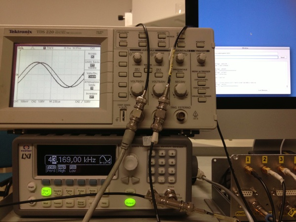
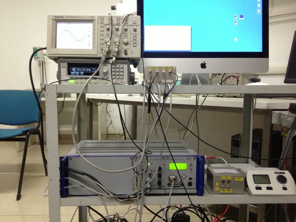
Setup of the Nanopositioning System


Viewing of the results of the scanned area


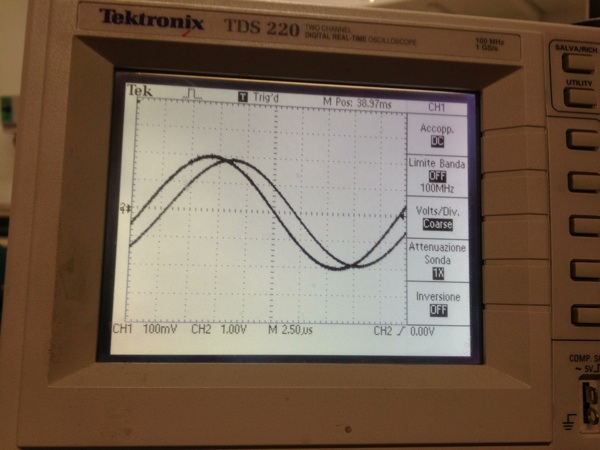
Viewing of the phase-difference of tension IN and OUT
by means of oscilloscope


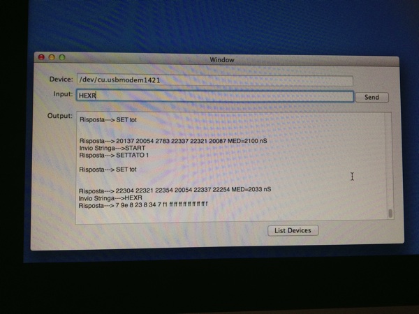
Viewing of the phase-difference of tension IN and OUT
by means of SW and Registration of the results in Memory